
Join me EVERY FRIDAY for #formulafriday and EVERY MONDAY for #macromondays on the http://www.howtoexcelatexcel.com blog for lots of #exceltips
Join thousands of other Excel users who have already joined the Excel At Excel Monthly Newsletter. 3 FREE Excel Tips every month.
http://www.howtoexcelatexcel.com/newsletter-sign-up/
Be Social & Let’s Connect
++Website http://www.howtoexcelatexcel.com
++Twitter https://twitter.com/howtoexcelatex
++Pinterest http://www.pinterest.com/howtoexcelat
#exceltips
#exceltipsandtricks
#exceltutorial
#exceltipsandtricks
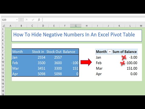
Hello Excellers, I have a handy Excel Pivot Table Tip for you today. I was creating a Pivot Table this week, (one of many!), and it contained negative numbers. Now, this was not the end of the world, but I really only wanted positive numbers to show in my Pivot Table. I did not want either of the zeros or the negative numbers to be visible. This is a handy little Excel trick, so I thought I would share it with you.
We can use cell formatting to hide both of the negative and zero numbers.
-Click on the Sum of Stock Balance field
-Click on Value Field Settings
-Number Formats
-Custom
-Special
-Type the following in the dialogue box 0;;;
-Hit Ok
*How Does The Custom Number Formatting Work In Excel?.*
So just how does that customer number formatting work in Excel?.
We need to first understand how Excel applies its number formatting.
Number formatting has up to four parts to it, all separated by semicolons. These code sections define the format for positive numbers, negative numbers, zero values, and text, in that specific order.
positive;negative;zero;text
So, in our example, we are leaving the positive numbers visible 0 but hiding the negative numbers by using a semicolon (;) as well as zero and text. You do not need to add the semicolons for all of the custom number formattings. For example, if we only wanted to specify two code sections the first is used for positive numbers and the second for negative numbers. If you only use one customer number format then it is used for all of the numbers.
If you want to use a number formatting for positive, skip negative then use formatting for zeros then you must include the ending semicolon for the section you skip. For example, let’s switch things up a bit and hide positive numbers and zeros, but allow negative numbers and if the cell contains text then display ‘this is text’. The custom formatting would be as below.
;-0;;“this is text”
You do not have to include all code sections in your custom number format. If you specify only two code sections for your custom number format, the first section is used for positive numbers and zeros, and the second section is used for negative numbers. If you specify only one code section, it is used for all numbers. So, you want to skip a code section and include a code section that follows it, you must include the ending semicolon for the section that you skip.
Final Formatting Of The Pivot Table.
To finish off the Pivot Table I removed the Grand Totals from the columns, as it is not relevant in or representative of the stock levels.
Right Click on the Pivot Table
Pivot Table Options
Totals & Filters
Untick Show Grand Totals For Columns